CEMENT ADVANCED PROCESS CONTROLS

Advanced Process Controls 100%

APC PERFORMANCE METRIC BENEFITS COMPUTATION SALES TOOL KIT

Top News

Click the button above to understand the step by step logic behind the APC Performance Metrics Benefit computation using Python3

CONTENTS

  • About Advanced Process Controls in Cement
  • What is this Cement APC Tool Kit?
  • What is Standard Deviation
  • What is Mean
  • What is Probability Density Function?
  • What are Z scores or Z-Transforms?
  • Application of Probability Density function and Z-scores to determine the distribution of Cement Feed using python
  • Tool Kit in Action

ADVANCED PROCESS CONTROLS IN CEMENT INDUSTRY


              The advent of APC that delivers the perfect combination – maximizing throughput and saving energy costs while meeting operational constraints resulting in significant increase in profitability – has brought about a revolution in the process industry. Previously, if a company selected APC, it had to heavily rely on highly experienced specialists to perform time-consuming tasks for maintaining and utilizing the technology. These engineers also had to spend a huge amount of time with less sophisticated tools in an attempt to better control plant behavior, which was not optimal because of the lack of leading-edge software.

It is critical to operate a plant safely and prevent production disruption, optimized operation is equally important. Change occurs constantly as stock pile composition and ambient conditions alter. Each change that occurs makes an impact on production, and hence the aim is to manage variables to achieve the right quality and quantity of the product required. If the predictive behavior of a plant is known, one can take appropriate measures on time to keep the plant at the optimal target.

The plant operators are not in a position to manually react to such changes and conduct corrective actions on a minute-by-minute basis and in an optimal way. APC enables manufacturers to resolve these issues. It can be applied to any process where outputs can be optimized on-line and in real-time, and any shop floor that has a distributed control system or programmable logic controls in place and where it is possible to model the dynamic predictive behavior of the plant.

APC implementation offers several benefits; for example, it improves process safety and reduces environmental emissions. Moreover, by reducing process variability, it will be possible to operate plants at their designed capacity. The software automatically improves operational efficiency; maximizes process profitability and business competitiveness; reduces cost, maintenance time and disruption through real-time asset optimization; and delivers improved visibility and decision support.


             The Advanced Process Controls System for Raw Mill, Kiln and Cement Mill will be interconnected to the control system of the plant. Hence the process measurement parameters like draft pressure, temperature, Mill power, Elevator load etc will be available for control. The Control Actions of the Actuators will be decided by the APC system based on the strategy of plant operation. Model Predictive controls is a methodology, where the entire process control system is modeled, by considering their system gain, time delay and time constant. After proper tuning of measurement weights and Actuator control actions, the APC control system takes control actions based on the predicted error between the measurement and its target current over the Prediction Horizon and also based on the controllers past actions. So, in short the APC system writes and reads set points to control system and which in turn controls the plant. A brief highlight on the working of APC is mentioned below:-

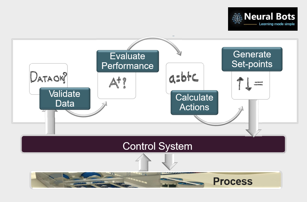
  • APC system reads the process measurements and the data is checked for its validations limits.
  • APC will then evaluate the process conditions by comparing the measurements with its stability targets.
  • Model Predictive Controller, which is one the main controllers, behind an APC system is used, to decide the quantum of action, which is then fine tuned, by adjusting the Modelling parameters of MPC, defined during formulating the strategy ,
  • The Set-Points for the Actuators generated by MPC are written back to the plant control system. This process happens every scan time defined by an APC system

Note: This Blog post although gives an introduction about APC in  Cement Industry but is more focused on the methodology and development of  “APC Performance Metric Benefit Computation” tool kit.

  • Model Predictive Controller is required to maintain the measurements on their assigned stability targets based on their weights.
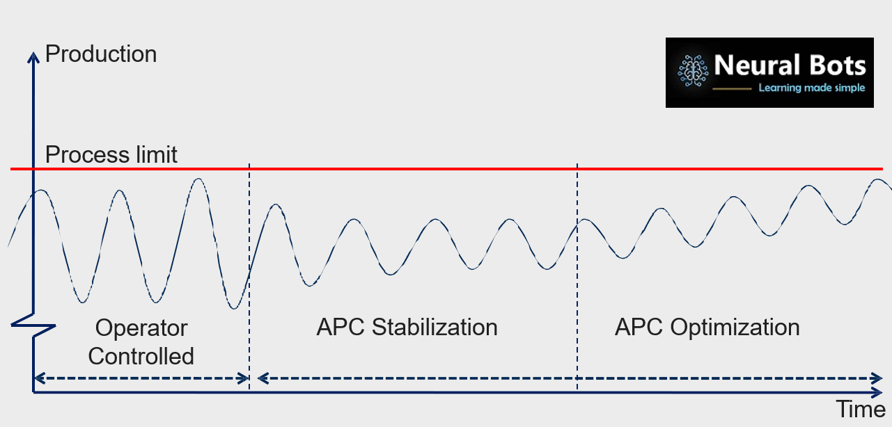
  • Based on the tuning of a MPC, stabilizing the process is primary goal of an APC system.
  • After Stabilization, APC system using different control techniques like Fuzzy Logic algorithm or using user defined control, tries to push the production targets to the maximum, thereby realizing the full potential of the process
  • Consistency in maintaining the process stability is the key metric of an APC system.

This is was all about the APC in action, in brief. But from selling point of view, what are the key metrics that needs analysis?

  • Firstly the Data set of the Mill or Kiln operation in offline mode for a period of one month (minimum) is required. ( The operators shouldn’t be aware the data was being recorded for this purpose so as even the play field)
  • For a Ball Mill, the main parameters were the Mill Feed (Actuator), Elevator Load, Mill Sound, Mill Power, Rejects, Outlet Temperature, Blaine as Stability Measurements will be available in the dataset.
  • So, the average, maximum and minimum statistics of these parameters gives us an idea about the operation of Mills/ Kiln. 
  • Based on the Power Margin available in the Mills / Kilns and source of material, a Production benefit and Specific Power Reduction benefit has to be decided.  These are the two Key selling parameters, which has to be demonstrated during execution.

How to determine the production and Specific Power benefit Parameters?

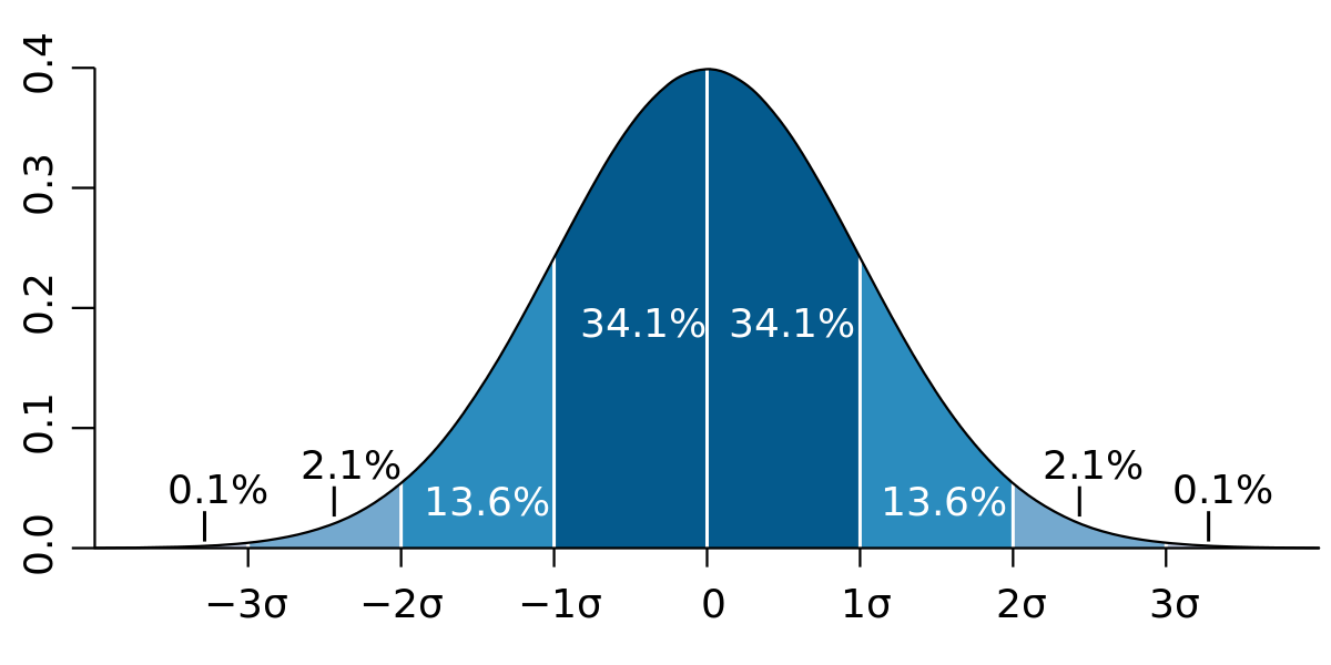
The Cement APC Tool Kit is designed to determine the potential benefit parameters of Production increase % and Specific Power reduction % using the concept of Probability Density Function and Z Scores. The details will be explained in the preceding section.


                             You guys know what is a mean mathematically. An average of a set of numbers in a dataset . You add up the numbers, divide by the number of items and Voila! you get the average. For example, the average of  Ball Mill Feed 206, 210 and 220 is:

206 + 210 + 220 =  636/ 3 = 212.

The you started studying statistics and all of a sudden the “average” is now called the mean. What happened? The answer is that they have the same meaning (they are synonyms).

The mean, or average, is represented by μ

That said, technically, the word mean is short for the arithmetic mean. We use different words in stats, because there are multiple different types of means, and they all do different things. 

For now you should be clear what is a mean!


What is Standard Deviation?


                          Standard deviation is a measure of dispersement in statistics. “Dispersement” tells you how much your data is spread out. Specifically, it shows you how much your data is spread out around the mean or average.

For example, when operator runs a mill for a week and you analyze the data. Standard Deviation gives you an idea how stable the Mill ran?. It also gives insights on the prevalence of disturbance in your process. It gives idea on the distribution of the samples of data around the mean!


How to visualize the standard deviation of the Ball Mill Feed samples distributed over a period of one month? 

Image Source :- Wikipedia

             The bell curve  or a “normal distribution“ is statistical tool to understand standard deviation.

The following graph of a normal distribution represents a great deal of data in real life. The mean, or average, is represented by μ, in the center. Each segment (colored in dark blue to light blue) represents one standard deviation away from the mean. For example, 2σ means two standard deviations from the mean.

A normal distribution curve can represent hundreds of situations in real life. 

After plotting a normal distribution curve for a Ball Mill Feed or Kiln Feed, you can pretty much visualize the distribution of feed. You can understand visually the deviations of samples from the mean.

Considering an instance, You’ll be able to predict that 34.1 + 34.1 = 68.2% of Ball Mill feed were distributed, very close to the average value, or one standard deviation away from the mean. 

Simple right?

This understanding can be potentially utilized to predict the  “Performance Metrics” as a selling parameter. It shows us visually, the places for improvements in brief!


              z-score a.k.a standard score gives you an idea of how far from the mean a data sample is present. But more technically, it’s a measure of how many standard deviations, a sample is placed below or above the mean.

A z-score can be placed on a normal distribution curve. Z-scores range from -3 standard deviations (which would fall to the far left of the normal distribution curve) up to +3 standard deviations (which would fall to the far right of the normal distribution curve). In order to use a z-score, you need to know the mean μ and also the population standard deviation σ.

Z-scores are a way to compare results to a “normal” population.

Now let’s apply this concept to analyze the Ball Mill Feed Samples. Let’s say you have a dataset of a cement mill with dependent and independent variables, let’s consider and analyze the Mill Feed. 

Let’s say the Mill was in continuous operation for a month and we can compute the Z-scores for the Mill Feed. This is to understand the spatial distribution of feed from the average value.

Average value denotes the operation comprising all the shift operations A, B , C or A/ B. Z- scores tells you the best feed runs in a sample of data and their % of distribution in the samples. 

A z-score can tell you where a particular feed sample is compared to the mean.

The basic z score formula for a feed sample is:

z = (x – μ) / σ

For example, let’s say you have a feed of 216 tph. The mean (μ) of 207.5 tph and a standard deviation (σ) of 25. Assuming a normal distribution, your z score would be:

  • Z = (x – μ) / σ
  • Z = (216 – 212.5) / 2.96 = 1.18 

The z score tells you how many standard deviations from the mean your score is. In this example, your score is 2.87 standard deviations above the mean.

Step 1: Write your X-value into the z-score equation. For this case we’ll enter the feed sample of interest or under observation which is 216 tph

  • Z = (216 – μ) / σ

Step 2: Put the mean, μ, into the z-score equation.

  • Z = (216 – 212.5) / σ

Step 3: Write the standard deviation, σ into the z-score equation.

  • Z = (216 – 212.5) / 2.96

           Z- Score = 1.18

Step 4: Look up your z-score in the z-table to see what percentage of feed samples fall below 216 tph.

i.e a Z-score of  1.18 is 0.3810 ( from Z-table right highlighted in red) + 0.5000 = 88.1 %

So, 88.1% of feed samples fall below the feed 216 tph or to the left under observation.

Inference:- 

           By computing the Z-scores, we place all the Feed samples in a standard scale of range -3 to +3 with μ = 0 and σ = 1,  which forms the foundation of standard normal distribution

Attached the Z-table for Reference:-

Z-table Right:-

Z

0.00

0.01

0.02

0.03

0.04

0.05

0.06

0.07

0.08

0.09

0.0

0.0000

0.0040

0.0080

0.0120

0.0160

0.0199

0.0239

0.0279

0.0319

0.0359

0.1

0.0398

0.0438

0.0478

0.0517

0.0557

0.0596

0.0636

0.0675

0.0714

0.0753

0.2

0.0793

0.0832

0.0871

0.0910

0.0948

0.0987

0.1026

0.1064

0.1103

0.1141

0.3

0.1179

0.1217

0.1255

0.1293

0.1331

0.1368

0.1406

0.1443

0.1480

0.1517

0.4

0.1554

0.1591

0.1628

0.1664

0.1700

0.1736

0.1772

0.1808

0.1844

0.1879

0.5

0.1915

0.1950

0.1985

0.2019

0.2054

0.2088

0.2123

0.2157

0.2190

0.2224

0.6

0.2257

0.2291

0.2324

0.2357

0.2389

0.2422

0.2454

0.2486

0.2517

0.2549

0.7

0.2580

0.2611

0.2642

0.2673

0.2704

0.2734

0.2764

0.2794

0.2823

0.2852

0.8

0.2881

0.2910

0.2939

0.2967

0.2995

0.3023

0.3051

0.3078

0.3106

0.3133

0.9

0.3159

0.3186

0.3212

0.3238

0.3264

0.3289

0.3315

0.3340

0.3365

0.3389

1.0

0.3413

0.3438

0.3461

0.3485

0.3508

0.3531

0.3554

0.3577

0.3599

0.3621

1.1

0.3643

0.3665

0.3686

0.3708

0.3729

0.3749

0.3770

0.3790

0.3810

0.3830

1.2

0.3849

0.3869

0.3888

0.3907

0.3925

0.3944

0.3962

0.3980

0.3997

0.4015

1.3

0.4032

0.4049

0.4066

0.4082

0.4099

0.4115

0.4131

0.4147

0.4162

0.4177

1.4

0.4192

0.4207

0.4222

0.4236

0.4251

0.4265

0.4279

0.4292

0.4306

0.4319

1.5

0.4332

0.4345

0.4357

0.4370

0.4382

0.4394

0.4406

0.4418

0.4429

0.4441

1.6

0.4452

0.4463

0.4474

0.4484

0.4495

0.4505

0.4515

0.4525

0.4535

0.4545

1.7

0.4554

0.4564

0.4573

0.4582

0.4591

0.4599

0.4608

0.4616

0.4625

0.4633

1.8

0.4641

0.4649

0.4656

0.4664

0.4671

0.4678

0.4686

0.4693

0.4699

0.4706

1.9

0.4713

0.4719

0.4726

0.4732

0.4738

0.4744

0.4750

0.4756

0.4761

0.4767

2.0

0.4772

0.4778

0.4783

0.4788

0.4793

0.4798

0.4803

0.4808

0.4812

0.4817

2.1

0.4821

0.4826

0.4830

0.4834

0.4838

0.4842

0.4846

0.4850

0.4854

0.4857

2.2

0.4861

0.4864

0.4868

0.4871

0.4875

0.4878

0.4881

0.4884

0.4887

0.4890

2.3

0.4893

0.4896

0.4898

0.4901

0.4904

0.4906

0.4909

0.4911

0.4913

0.4916

2.4

0.4918

0.4920

0.4922

0.4925

0.4927

0.4929

0.4931

0.4932

0.4934

0.4936

2.5

0.4938

0.4940

0.4941

0.4943

0.4945

0.4946

0.4948

0.4949

0.4951

0.4952

2.6

0.4953

0.4955

0.4956

0.4957

0.4959

0.4960

0.4961

0.4962

0.4963

0.4964

2.7

0.4965

0.4966

0.4967

0.4968

0.4969

0.4970

0.4971

0.4972

0.4973

0.4974

2.8

0.4974

0.4975

0.4976

0.4977

0.4977

0.4978

0.4979

0.4979

0.4980

0.4981

2.9

0.4981

0.4982

0.4982

0.4983

0.4984

0.4984

0.4985

0.4985

0.4986

0.4986

3.0

0.4987

0.4987

0.4987

0.4988

0.4988

0.4989

0.4989

0.4989

0.4990

0.4990

3.1

0.4990

0.4991

0.4991

0.4991

0.4992

0.4992

0.4992

0.4992

0.4993

0.4993

3.2

0.4993

0.4993

0.4994

0.4994

0.4994

0.4994

0.4994

0.4995

0.4995

0.4995

3.3

0.4995

0.4995

0.4995

0.4996

0.4996

0.4996

0.4996

0.4996

0.4996

0.4997

3.4

0.4997

0.4997

0.4997

0.4997

0.4997

0.4997

0.4997

0.4997

0.4997

0.4998

3.5

0.4998

0.4998

0.4998

0.4998

0.4998

0.4998

0.4998

0.4998

0.4998

0.4998

3.6

0.4998

0.4998

0.4999

0.4999

0.4999

0.4999

0.4999

0.4999

0.4999

0.4999

3.7

0.4999

0.4999

0.4999

0.4999

0.4999

0.4999

0.4999

0.4999

0.4999

0.4999

3.8

0.4999

0.4999

0.4999

0.4999

0.4999

0.4999

0.4999

0.4999

0.4999

0.4999

 Z-table Left:-

Z

0.00

0.01

0.02

0.03

0.04

0.05

0.06

0.07

0.08

0.09

0.0

0.5000

0.5040

0.5080

0.0120

0.0160

0.0199

0.5239

0.0279

0.0319

0.0359

0.1

0.5398

0.5438

0.5478

0.5517

0.5557

0.5596

0.5636

0.5675

0.5714

0.5753

0.2

0.5793

0.5832

0.5871

0.5910

0.5948

0.5987

0.6064

0.1064

0.6103

0.6141

0.3

0.6179

0.6217

0.6255

0.6293

0.6331

0.6368

0.6406

0.6443

0.6480

0.6517

0.4

0.6554

0.6591

0.6628

0.6664

0.6700

0.6736

0.6772

0.6808

0.6844

0.6879

0.5

0.6915

0.6950

0.6985

0.7019

0.7054

0.7088

0.7123

0.7157

0.7190

0.7224

0.6

0.7257

0.7291

0.7324

0.7357

0.7389

0.7422

0.7454

0.7486

0.7517

0.7549

0.7

0.7580

0.7611

0.7642

0.7673

0.7704

0.7734

0.7764

0.7794

0.7823

0.7852

0.8

0.7881

0.7910

0.7939

0.7967

0.7995

0.8023

0.8051

0.8078

0.8106

0.8133

0.9

0.8159

0.8186

0.8212

0.8238

0.8264

0.8289

0.8315

0.8340

0.8365

0.8389

1.0

0.8413

0.8438

0.8461

0.8485

0.8508

0.8531

0.8554

0.8577

0.8599

0.8621

1.1

0.8643

0.8665

0.8686

0.8708

0.8729

0.8749

0.8770

0.8790

0.8810

0.8830

1.2

0.8849

0.8869

0.8888

0.8907

0.8925

0.8944

0.8962

0.8980

0.8997

0.9015

1.3

0.9032

0.9049

0.9066

0.9082

0.9099

0.9115

0.9131

0.9147

0.9162

0.9177

1.4

0.9192

0.9207

0.9222

0.9236

0.9251

0.9265

0.9279

0.9292

0.9306

0.9319

1.5

0.9332

0.9345

0.9357

0.9370

0.9382

0.9394

0.9406

0.9418

0.9429

0.9441

1.6

0.9452

0.9463

0.9474

0.9484

0.9495

0.9505

0.9515

0.9525

0.9535

0.9545

1.7

0.9554

0.9564

0.9573

0.9582

0.9591

0.9599

0.9608

0.9616

0.9625

0.9633

1.8

0.9641

0.9649

0.9656

0.9664

0.9671

0.9678

0.9686

0.9693

0.9699

0.9706

1.9

0.9713

0.9719

0.9726

0.9732

0.9738

0.9744

0.9750

0.9756

0.9761

0.9767

2.0

0.9772

0.9778

0.9783

0.9788

0.9793

0.9798

0.9803

0.9808

0.9812

0.9817

2.1

0.9821

0.9826

0.9830

0.9834

0.9838

0.9842

0.9846

0.9850

0.9854

0.9857

2.2

0.9861

0.9864

0.9868

0.9871

0.9875

0.9878

0.9881

0.9884

0.9887

0.9890

2.3

0.9893

0.9896

0.9898

0.9901

0.9904

0.9906

0.9909

0.9911

0.9913

0.9916

2.4

0.9918

0.9920

0.9922

0.9925

0.9927

0.9929

0.9931

0.9932

0.9934

0.9936

2.5

0.9938

0.9940

0.9941

0.9943

0.9945

0.9946

0.9948

0.9949

0.9951

0.9952

2.6

0.9953

0.9955

0.9956

0.9957

0.9959

0.9960

0.9961

0.9962

0.9963

0.9964

2.7

0.9965

0.9966

0.9967

0.9968

0.9969

0.9970

0.9971

0.9972

0.9973

0.9974

2.8

0.9974

0.9975

0.9976

0.9977

0.9977

0.9978

0.9979

0.9979

0.9980

0.9981

2.9

0.9981

0.9982

0.9982

0.9983

0.9984

0.9984

0.9985

0.9985

0.9986

0.9986

3.0

0.9987

0.9987

0.9987

0.9988

0.9988

0.9989

0.9989

0.9989

0.9990

0.9990

 Note:-

Why add .500 to the result? The z-table shown has scores for the RIGHT of the mean. Therefore, we have to add .500 for all of the area LEFT of the mean. So you have to subtract 0.5 if any sample is analyzed to the left of mean.

Area under a normal distribution curve.+ .5000 =  0.881 or 88.1%.


The general formula for the probability density function of the normal distribution is

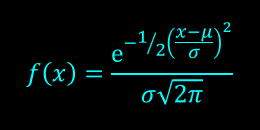
μ is the location parameter and σ is the scale parameter.

The case where μ = 0 and σ = 1 after computing the Z-scores is called the standard normal distribution

Equation for the standard normal distribution is

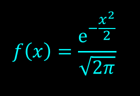
The following is the plot of the standard normal probability density function.

Click the button above to understand the step by step logic behind the APC Performance Metrics Benefit computation using Python3

Alright, before we jump into experimenting the Probability Density Function, to use this toolkit effectively, you can follow the rules below:-

  • The Dataset of Raw Mill/ Cement Mill/ Kiln should be pre-processed as per the format. Screenshot reference available in the image below.
  • The Features or the columns can be in any order.
  • There should be a single header specifying the descriptions of the dependent and independent variables.
  • Avoid adding spaces between two words and avoid adding units  Eg:- Avoid “Elevator Load” instead try as “Elevator_Load” (This is because the program is designed and standardized to handle most of the dataset from Cement )
  • Make sure the Mill Feed or the kiln feed column description should be renamed as “Total_Feed”.
  • Before you upload the dataset in the site, rename the dataset,  you want to analyze as ‘CementAPCToolKit_RawMill.csv’ or ‘CementAPCToolKit_CoalMill.csv’ or ‘CementAPCToolKit_Kiln.csv’ or ‘CementAPCToolKit_CementMill.csv’
  • Browse for the pre-processed dataset by clicking on the Select file button
  • Click on Upload
  • After successful upload, run the python program by clicking on “Run”
  • After then you will be prompted to enter the section of plant for which the dataset needs analysis. Enter them as RawMill or CoalMill or Kiln or CementMill, the same suffix as you just uploaded.
  • Enjoy the Analysis.

Note:- If you face issues using this toolkit go to — Contact — Fill the Contact Form, I’ll get back to you!  You can also reach out to me by sending your queries on [email protected]