The advent of APC that delivers the perfect combination – maximizing throughput and saving energy costs while meeting operational constraints resulting in significant increase in profitability – has brought about a revolution in the process industry. Previously, if a company selected APC, it had to heavily rely on highly experienced specialists to perform time-consuming tasks for maintaining and utilizing the technology. These engineers also had to spend a huge amount of time with less sophisticated tools in an attempt to better control plant behavior, which was not optimal because of the lack of leading-edge software.
It is critical to operate a plant safely and prevent production disruption, optimized operation is equally important. Change occurs constantly as stock pile composition and ambient conditions alter. Each change that occurs makes an impact on production, and hence the aim is to manage variables to achieve the right quality and quantity of the product required. If the predictive behavior of a plant is known, one can take appropriate measures on time to keep the plant at the optimal target.
The plant operators are not in a position to manually react to such changes and conduct corrective actions on a minute-by-minute basis and in an optimal way. APC enables manufacturers to resolve these issues. It can be applied to any process where outputs can be optimized on-line and in real-time, and any shop floor that has a distributed control system or programmable logic controls in place and where it is possible to model the dynamic predictive behavior of the plant.
APC implementation offers several benefits; for example, it improves process safety and reduces environmental emissions. Moreover, by reducing process variability, it will be possible to operate plants at their designed capacity. The software automatically improves operational efficiency; maximizes process profitability and business competitiveness; reduces cost, maintenance time and disruption through real-time asset optimization; and delivers improved visibility and decision support.
The Advanced Process Controls System for Raw Mill, Kiln and Cement Mill will be interconnected to the control system of the plant. Hence the process measurement parameters like draft pressure, temperature, Mill power, Elevator load etc will be available for control. The Control Actions of the Actuators will be decided by the APC system based on the strategy of plant operation. Model Predictive controls is a methodology, where the entire process control system is modeled, by considering their system gain, time delay and time constant. After proper tuning of measurement weights and Actuator control actions, the APC control system takes control actions based on the predicted error between the measurement and its target current over the Prediction Horizon and also based on the controllers past actions. So, in short the APC system writes and reads set points to control system and which in turn controls the plant. A brief highlight on the working of APC is mentioned:-
Note: This Blog post although gives an introduction about APC in Cement Industry but is more focused on the methodology and development of “APC Performance Metric Benefit Computation” tool kit.
This is was all about the APC in action, in brief. But from selling point of view, what are the key metrics that needs analysis?
How to determine the production and Specific Power benefit Parameters?
The Cement APC Tool Kit is designed to determine the potential benefit parameters of Production increase % and Specific Power reduction % using the concept of Probability Density Function and Z Scores. The details will be explained in the preceding section.
The mean—often simply called the average—is a measure of the “central” value of a collection of numbers. More precisely:
Arithmetic mean
Given a set of nn numbers {x1,x2,…,xn}{x1,x2,…,xn}, the arithmetic mean is
xˉ = 1n∑i=1nxixˉ=n1i=1∑nxi
You add up all the values, then divide by how many there are.
Notation
When referring to a population mean (every member of some group), we often use the Greek letter μμ.
When referring to a sample mean (a subset or sample from a population), we write xˉxˉ.
In everyday language “average” can mean various things (mean, median, mode, etc.), but in mathematics and statistics:
Mean (short for arithmetic mean) is one specific kind of average.
There are other “means” (e.g., geometric mean, harmonic mean) each suited to different contexts.
Say you have three measurements of Ball Mill feed rates:
206,210,220.206,210,220.
Their arithmetic mean is
xˉ = 206+210+2203 = 6363 = 212.xˉ=3206+210+220=3636=212.
So the “average” feed rate is 212.
Name | Formula for nn positive values xixi | Use-case |
---|---|---|
Geometric mean | (∏i=1nxi)1/n(i=1∏nxi)1/n | Growth rates (e.g., finance, biology) |
Harmonic mean | n∑i=1n1xi∑i=1nxi1n | Rates and ratios (e.g., speeds, densities) |
Each “mean” answers a slightly different question about the data’s central tendency.
Mean = average (in the arithmetic‐sense).
Notation: μμ for populations, xˉxˉ for samples.
There are multiple “means” beyond the arithmetic one; use the one appropriate for your data.
Standard deviation is a measure of how “spread out” or dispersed a set of values is around their mean (average). In more precise terms:
Population standard deviation (σ)
When you have data for an entire population of size NN, the standard deviation is
σ = 1N∑i=1N(xi−μ)2σ=N1i=1∑N(xi−μ)2
where
xixi are the individual data points,
μ=1N∑i=1Nxiμ=N1∑i=1Nxi is the population mean.
Sample standard deviation (s)
When your data are a sample of size nn drawn from a larger population, you use
s = 1n−1∑i=1n(xi−xˉ)2s=n−11i=1∑n(xi−xˉ)2
where
xˉ=1n∑i=1nxixˉ=n1∑i=1nxi is the sample mean,
dividing by n−1n−1 (instead of nn) corrects for the fact that xˉxˉ itself is estimated from the data.
Deviation of each point: xi−μxi−μ.
If you simply summed deviations, positive and negative differences would cancel out to zero.
Squaring each deviation makes all terms non-negative, so you get a true measure of overall spread.
Taking the square root at the end returns the measure to the same units as the original data.
Suppose you measure Ball Mill feed rates:
206,210,220.206,210,220.
Mean: μ=(206+210+220)/3=212μ=(206+210+220)/3=212.
Deviations from the mean:
206−212=−6,210−212=−2,220−212=+8.206−212=−6,210−212=−2,220−212=+8.
Squared deviations:
(−6)2=36,(−2)2=4,82=64,sum=104.(−6)2=36,(−2)2=4,82=64,sum=104.
Variance (population):
σ2=1043≈34.67.σ2=3104≈34.67.
Standard deviation:
σ=34.67≈5.89.σ=34.67≈5.89.
So on average, feed‐rate measurements deviate about 5.9 units from the mean of 212.
For data that follow (or approximately follow) a normal (bell-shaped) distribution:
About 68% of values lie within one standard deviation of the mean (μ±1σμ±1σ).
About 95% lie within two standard deviations (μ±2σμ±2σ).
About 99.7% lie within three standard deviations (μ±3σμ±3σ).
Visually, each “band” around the center captures a fixed percentage of the total area under the curve:
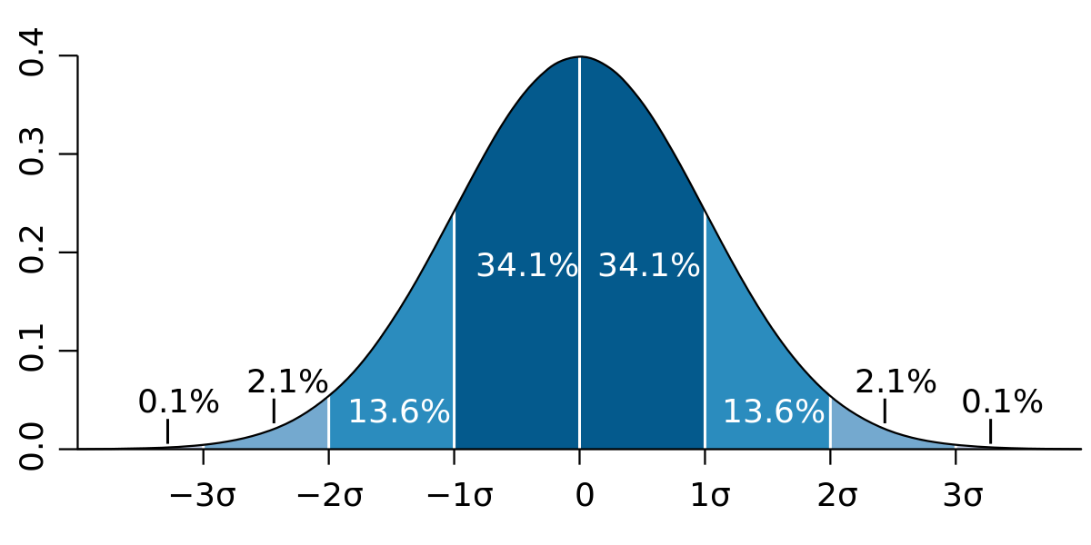
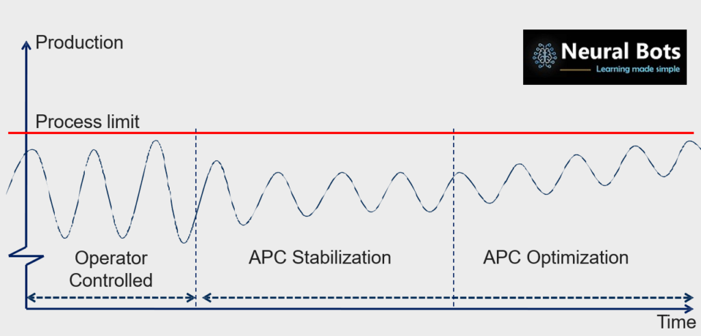
Stability: A small standard deviation means your process (e.g., mill feed rate) is consistently near its average—good for quality control.
Disturbances: A large standard deviation signals frequent or large deviations—points toward process disturbances or variability.
By tracking standard deviation over time, you can pinpoint when a process is “drifting” or becoming more erratic, and take corrective action.
Standard deviation quantifies average distance from the mean.
Population vs. sample formulas differ only in the denominator (NN vs. n−1n−1).
In a normal distribution, σ has clear probabilistic interpretations (68–95–99.7 rule).
Monitoring σ helps you assess and improve process stability.
A z-score (or standard score) tells you exactly how many standard deviations a data point lies from the mean of its distribution. In other words, it “standardizes” any value xx by translating and scaling it relative to the population’s average (μμ) and dispersion (σσ):
z=x−μσ z=σx−μ
If z=0z=0, the point is exactly at the mean.
If z=+2z=+2, it’s two standard deviations above the mean.
If z=−1.5z=−1.5, it’s 1.5 standard deviations below the mean.
By converting to this common scale (mean = 0, σ = 1), you can compare values from different datasets or read probabilities directly off the standard normal curve.
On a bell-shaped (normal) distribution:
About 68% of values fall between z=−1z=−1 and z=+1z=+1.
About 95% lie between z=−2z=−2 and z=+2z=+2.
About 99.7% lie between z=−3z=−3 and z=+3z=+3.
A z-table (or cumulative normal table) gives you the area to the left (or right) of any zz-value.
Suppose over a month your mill’s feed data have:
Mean μ=212.5 tphμ=212.5 tph
Standard deviation σ=2.96 tphσ=2.96 tph
You observe one shift’s feed at x=216 tphx=216 tph. Its z-score is
z=216−212.52.96 ≈ 1.18.z=2.96216−212.5≈1.18.
Interpretation: That run was 1.18 σ above the month’s average.
Percentile: Looking up z=1.18z=1.18 on the standard normal table gives a cumulative area of about 0.881 (or 88.1%) to the left of that point.
In practice: roughly 88.1% of all feed samples fall at or below 216 tph.
Benchmarking: You can compare any feed reading to the entire month’s performance on a common scale.
Outlier detection: Runs with ∣z∣>2∣z∣>2 or 3 are statistically rare—prime suspects for equipment issues or feed disturbances.
Probability insights: Z-scores directly map to probabilities, so you know how unusual any particular observation is.
By routinely converting your feed data to z-scores, you turn raw tph readings into a standardized, probability-based framework—making patterns, drifts, and outliers immediately visible.
Attached the Z-table for Reference:-
Z-table Right:-
Z | 0.00 | 0.01 | 0.02 | 0.03 | 0.04 | 0.05 | 0.06 | 0.07 | 0.08 | 0.09 |
---|---|---|---|---|---|---|---|---|---|---|
0.0 | 0.0000 | 0.0040 | 0.0080 | 0.0120 | 0.0160 | 0.0199 | 0.0239 | 0.0279 | 0.0319 | 0.0359 |
0.1 | 0.0398 | 0.0438 | 0.0478 | 0.0517 | 0.0557 | 0.0596 | 0.0636 | 0.0675 | 0.0714 | 0.0753 |
0.2 | 0.0793 | 0.0832 | 0.0871 | 0.0910 | 0.0948 | 0.0987 | 0.1026 | 0.1064 | 0.1103 | 0.1141 |
0.3 | 0.1179 | 0.1217 | 0.1255 | 0.1293 | 0.1331 | 0.1368 | 0.1406 | 0.1443 | 0.1480 | 0.1517 |
0.4 | 0.1554 | 0.1591 | 0.1628 | 0.1664 | 0.1700 | 0.1736 | 0.1772 | 0.1808 | 0.1844 | 0.1879 |
0.5 | 0.1915 | 0.1950 | 0.1985 | 0.2019 | 0.2054 | 0.2088 | 0.2123 | 0.2157 | 0.2190 | 0.2224 |
0.6 | 0.2257 | 0.2291 | 0.2324 | 0.2357 | 0.2389 | 0.2422 | 0.2454 | 0.2486 | 0.2517 | 0.2549 |
0.7 | 0.2580 | 0.2611 | 0.2642 | 0.2673 | 0.2704 | 0.2734 | 0.2764 | 0.2794 | 0.2823 | 0.2852 |
0.8 | 0.2881 | 0.2910 | 0.2939 | 0.2967 | 0.2995 | 0.3023 | 0.3051 | 0.3078 | 0.3106 | 0.3133 |
0.9 | 0.3159 | 0.3186 | 0.3212 | 0.3238 | 0.3264 | 0.3289 | 0.3315 | 0.3340 | 0.3365 | 0.3389 |
1.0 | 0.3413 | 0.3438 | 0.3461 | 0.3485 | 0.3508 | 0.3531 | 0.3554 | 0.3577 | 0.3599 | 0.3621 |
1.1 | 0.3643 | 0.3665 | 0.3686 | 0.3708 | 0.3729 | 0.3749 | 0.3770 | 0.3790 | 0.3810 | 0.3830 |
1.2 | 0.3849 | 0.3869 | 0.3888 | 0.3907 | 0.3925 | 0.3944 | 0.3962 | 0.3980 | 0.3997 | 0.4015 |
1.3 | 0.4032 | 0.4049 | 0.4066 | 0.4082 | 0.4099 | 0.4115 | 0.4131 | 0.4147 | 0.4162 | 0.4177 |
1.4 | 0.4192 | 0.4207 | 0.4222 | 0.4236 | 0.4251 | 0.4265 | 0.4279 | 0.4292 | 0.4306 | 0.4319 |
1.5 | 0.4332 | 0.4345 | 0.4357 | 0.4370 | 0.4382 | 0.4394 | 0.4406 | 0.4418 | 0.4429 | 0.4441 |
1.6 | 0.4452 | 0.4463 | 0.4474 | 0.4484 | 0.4495 | 0.4505 | 0.4515 | 0.4525 | 0.4535 | 0.4545 |
1.7 | 0.4554 | 0.4564 | 0.4573 | 0.4582 | 0.4591 | 0.4599 | 0.4608 | 0.4616 | 0.4625 | 0.4633 |
1.8 | 0.4641 | 0.4649 | 0.4656 | 0.4664 | 0.4671 | 0.4678 | 0.4686 | 0.4693 | 0.4699 | 0.4706 |
1.9 | 0.4713 | 0.4719 | 0.4726 | 0.4732 | 0.4738 | 0.4744 | 0.4750 | 0.4756 | 0.4761 | 0.4767 |
2.0 | 0.4772 | 0.4778 | 0.4783 | 0.4788 | 0.4793 | 0.4798 | 0.4803 | 0.4808 | 0.4812 | 0.4817 |
2.1 | 0.4821 | 0.4826 | 0.4830 | 0.4834 | 0.4838 | 0.4842 | 0.4846 | 0.4850 | 0.4854 | 0.4857 |
2.2 | 0.4861 | 0.4864 | 0.4868 | 0.4871 | 0.4875 | 0.4878 | 0.4881 | 0.4884 | 0.4887 | 0.4890 |
2.3 | 0.4893 | 0.4896 | 0.4898 | 0.4901 | 0.4904 | 0.4906 | 0.4909 | 0.4911 | 0.4913 | 0.4916 |
2.4 | 0.4918 | 0.4920 | 0.4922 | 0.4925 | 0.4927 | 0.4929 | 0.4931 | 0.4932 | 0.4934 | 0.4936 |
2.5 | 0.4938 | 0.4940 | 0.4941 | 0.4943 | 0.4945 | 0.4946 | 0.4948 | 0.4949 | 0.4951 | 0.4952 |
2.6 | 0.4953 | 0.4955 | 0.4956 | 0.4957 | 0.4959 | 0.4960 | 0.4961 | 0.4962 | 0.4963 | 0.4964 |
2.7 | 0.4965 | 0.4966 | 0.4967 | 0.4968 | 0.4969 | 0.4970 | 0.4971 | 0.4972 | 0.4973 | 0.4974 |
2.8 | 0.4974 | 0.4975 | 0.4976 | 0.4977 | 0.4977 | 0.4978 | 0.4979 | 0.4979 | 0.4980 | 0.4981 |
2.9 | 0.4981 | 0.4982 | 0.4982 | 0.4983 | 0.4984 | 0.4984 | 0.4985 | 0.4985 | 0.4986 | 0.4986 |
3.0 | 0.4987 | 0.4987 | 0.4987 | 0.4988 | 0.4988 | 0.4989 | 0.4989 | 0.4989 | 0.4990 | 0.4990 |
3.1 | 0.4990 | 0.4991 | 0.4991 | 0.4991 | 0.4992 | 0.4992 | 0.4992 | 0.4992 | 0.4993 | 0.4993 |
3.2 | 0.4993 | 0.4993 | 0.4994 | 0.4994 | 0.4994 | 0.4994 | 0.4994 | 0.4995 | 0.4995 | 0.4995 |
3.3 | 0.4995 | 0.4995 | 0.4995 | 0.4996 | 0.4996 | 0.4996 | 0.4996 | 0.4996 | 0.4996 | 0.4997 |
3.4 | 0.4997 | 0.4997 | 0.4997 | 0.4997 | 0.4997 | 0.4997 | 0.4997 | 0.4997 | 0.4997 | 0.4998 |
3.5 | 0.4998 | 0.4998 | 0.4998 | 0.4998 | 0.4998 | 0.4998 | 0.4998 | 0.4998 | 0.4998 | 0.4998 |
3.6 | 0.4998 | 0.4998 | 0.4999 | 0.4999 | 0.4999 | 0.4999 | 0.4999 | 0.4999 | 0.4999 | 0.4999 |
3.7 | 0.4999 | 0.4999 | 0.4999 | 0.4999 | 0.4999 | 0.4999 | 0.4999 | 0.4999 | 0.4999 | 0.4999 |
3.8 | 0.4999 | 0.4999 | 0.4999 | 0.4999 | 0.4999 | 0.4999 | 0.4999 | 0.4999 | 0.4999 | 0.4999 |
Z-table Left:-
Z | 0.00 | 0.01 | 0.02 | 0.03 | 0.04 | 0.05 | 0.06 | 0.07 | 0.08 | 0.09 |
---|---|---|---|---|---|---|---|---|---|---|
0.0 | 0.5000 | 0.5040 | 0.5080 | 0.0120 | 0.0160 | 0.0199 | 0.5239 | 0.0279 | 0.0319 | 0.0359 |
0.1 | 0.5398 | 0.5438 | 0.5478 | 0.5517 | 0.5557 | 0.5596 | 0.5636 | 0.5675 | 0.5714 | 0.5753 |
0.2 | 0.5793 | 0.5832 | 0.5871 | 0.5910 | 0.5948 | 0.5987 | 0.6064 | 0.1064 | 0.6103 | 0.6141 |
0.3 | 0.6179 | 0.6217 | 0.6255 | 0.6293 | 0.6331 | 0.6368 | 0.6406 | 0.6443 | 0.6480 | 0.6517 |
0.4 | 0.6554 | 0.6591 | 0.6628 | 0.6664 | 0.6700 | 0.6736 | 0.6772 | 0.6808 | 0.6844 | 0.6879 |
0.5 | 0.6915 | 0.6950 | 0.6985 | 0.7019 | 0.7054 | 0.7088 | 0.7123 | 0.7157 | 0.7190 | 0.7224 |
0.6 | 0.7257 | 0.7291 | 0.7324 | 0.7357 | 0.7389 | 0.7422 | 0.7454 | 0.7486 | 0.7517 | 0.7549 |
0.7 | 0.7580 | 0.7611 | 0.7642 | 0.7673 | 0.7704 | 0.7734 | 0.7764 | 0.7794 | 0.7823 | 0.7852 |
0.8 | 0.7881 | 0.7910 | 0.7939 | 0.7967 | 0.7995 | 0.8023 | 0.8051 | 0.8078 | 0.8106 | 0.8133 |
0.9 | 0.8159 | 0.8186 | 0.8212 | 0.8238 | 0.8264 | 0.8289 | 0.8315 | 0.8340 | 0.8365 | 0.8389 |
1.0 | 0.8413 | 0.8438 | 0.8461 | 0.8485 | 0.8508 | 0.8531 | 0.8554 | 0.8577 | 0.8599 | 0.8621 |
1.1 | 0.8643 | 0.8665 | 0.8686 | 0.8708 | 0.8729 | 0.8749 | 0.8770 | 0.8790 | 0.8810 | 0.8830 |
1.2 | 0.8849 | 0.8869 | 0.8888 | 0.8907 | 0.8925 | 0.8944 | 0.8962 | 0.8980 | 0.8997 | 0.9015 |
1.3 | 0.9032 | 0.9049 | 0.9066 | 0.9082 | 0.9099 | 0.9115 | 0.9131 | 0.9147 | 0.9162 | 0.9177 |
1.4 | 0.9192 | 0.9207 | 0.9222 | 0.9236 | 0.9251 | 0.9265 | 0.9279 | 0.9292 | 0.9306 | 0.9319 |
1.5 | 0.9332 | 0.9345 | 0.9357 | 0.9370 | 0.9382 | 0.9394 | 0.9406 | 0.9418 | 0.9429 | 0.9441 |
1.6 | 0.9452 | 0.9463 | 0.9474 | 0.9484 | 0.9495 | 0.9505 | 0.9515 | 0.9525 | 0.9535 | 0.9545 |
1.7 | 0.9554 | 0.9564 | 0.9573 | 0.9582 | 0.9591 | 0.9599 | 0.9608 | 0.9616 | 0.9625 | 0.9633 |
1.8 | 0.9641 | 0.9649 | 0.9656 | 0.9664 | 0.9671 | 0.9678 | 0.9686 | 0.9693 | 0.9699 | 0.9706 |
1.9 | 0.9713 | 0.9719 | 0.9726 | 0.9732 | 0.9738 | 0.9744 | 0.9750 | 0.9756 | 0.9761 | 0.9767 |
2.0 | 0.9772 | 0.9778 | 0.9783 | 0.9788 | 0.9793 | 0.9798 | 0.9803 | 0.9808 | 0.9812 | 0.9817 |
2.1 | 0.9821 | 0.9826 | 0.9830 | 0.9834 | 0.9838 | 0.9842 | 0.9846 | 0.9850 | 0.9854 | 0.9857 |
2.2 | 0.9861 | 0.9864 | 0.9868 | 0.9871 | 0.9875 | 0.9878 | 0.9881 | 0.9884 | 0.9887 | 0.9890 |
2.3 | 0.9893 | 0.9896 | 0.9898 | 0.9901 | 0.9904 | 0.9906 | 0.9909 | 0.9911 | 0.9913 | 0.9916 |
2.4 | 0.9918 | 0.9920 | 0.9922 | 0.9925 | 0.9927 | 0.9929 | 0.9931 | 0.9932 | 0.9934 | 0.9936 |
2.5 | 0.9938 | 0.9940 | 0.9941 | 0.9943 | 0.9945 | 0.9946 | 0.9948 | 0.9949 | 0.9951 | 0.9952 |
2.6 | 0.9953 | 0.9955 | 0.9956 | 0.9957 | 0.9959 | 0.9960 | 0.9961 | 0.9962 | 0.9963 | 0.9964 |
2.7 | 0.9965 | 0.9966 | 0.9967 | 0.9968 | 0.9969 | 0.9970 | 0.9971 | 0.9972 | 0.9973 | 0.9974 |
2.8 | 0.9974 | 0.9975 | 0.9976 | 0.9977 | 0.9977 | 0.9978 | 0.9979 | 0.9979 | 0.9980 | 0.9981 |
2.9 | 0.9981 | 0.9982 | 0.9982 | 0.9983 | 0.9984 | 0.9984 | 0.9985 | 0.9985 | 0.9986 | 0.9986 |
3.0 | 0.9987 | 0.9987 | 0.9987 | 0.9988 | 0.9988 | 0.9989 | 0.9989 | 0.9989 | 0.9990 | 0.9990 |
Note:-
Why add .500 to the result? The z-table shown has scores for the RIGHT of the mean. Therefore, we have to add .500 for all of the area LEFT of the mean. So you have to subtract 0.5 if any sample is analyzed to the left of mean.
Area under a normal distribution curve.+ .5000 = 0.881 or 88.1%.
A probability density function f(x)f(x) for a continuous variable XX (e.g., kiln temperature, mill power draw, or feed rate) tells you how likely you are to observe any particular value xx. In APC you use PDFs to:
Characterize disturbances: Model feed variability or fuel‐quality swings that “disturb” your process.
Quantify uncertainty: In model‐predictive control (MPC), the controller propagates input and measurement uncertainties—often assuming they follow known PDFs (e.g., Gaussian).
Detect anomalies: Values falling in the tails of the PDF (very low density regions) flag unusual conditions or sensor faults.
Data collection
Gather high‐resolution time series of key process variables (e.g., mill load, separator pressure).
Histogram or Kernel Density
Histogram: Bin your measurements to approximate the PDF.
Kernel density estimation (KDE): Smooths the histogram into a continuous curve.
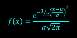
Fit a parametric form
Often a normal distribution is assumed:
f(x)=1σ2πexp (−(x−μ)22σ2).f(x)=σ2π1exp(−2σ2(x−μ)2).In many cement processes, data can be skewed—so you might fit a log‐normal or Weibull distribution instead.
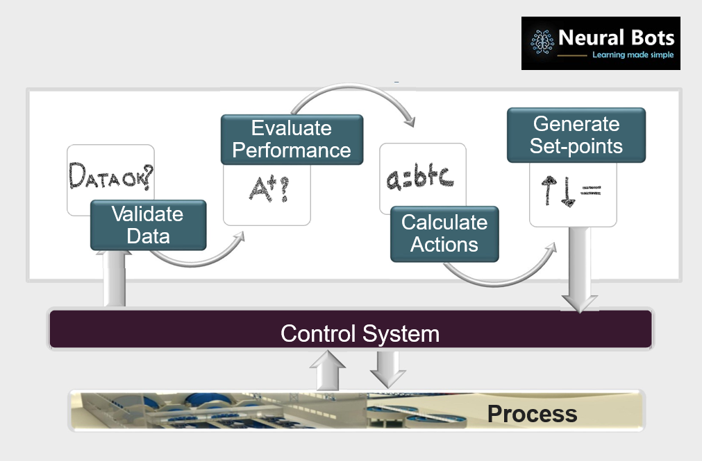
Modern APC systems in cement plants typically use MPC algorithms that:
Predict future process behavior over a horizon NN using a dynamic model.
Optimize a sequence of control moves (valve positions, mill speed) to minimize a cost function (e.g., deviation from target plus move‐effort).
When disturbances (like feed variation or fuel LHV) are modeled as random variables:
The controller uses their PDFs to propagate uncertainty through the model.
It can then perform chance‐constrained optimization, ensuring that constraints (e.g., maximum kiln shell temperature) are violated with only a small, acceptable probability (say 1%).
APC solutions often include soft sensors (statistical estimators) for hard‐to‐measure variables (like clinker quality). You:
Estimate the PDF of the soft‐sensor’s residual (estimation error).
Monitor incoming measured data versus the predicted PDF.
Alarm when the observed value falls in a region of extremely low density—indicating sensor drift or process upset.
Stability assessment: By comparing the real‐time PDF of mill power draw against its historical “normal” PDF, you can detect creeping variance (e.g., grinding media wear) before it impacts throughput.
Disturbance rejection: Knowing the distribution of raw‐feed moisture lets the APC tune the kiln’s fuel‐feed controller to compensate more aggressively when large deviations are likely.
Quality assurance: PDF‐based confidence intervals around predicted clinker free‐lime content inform operators when to sample the product.
PDFs translate raw data into probability statements—central to any statistical control or estimation algorithm in APC.
MPC uses PDFs to handle disturbance and measurement uncertainty, enabling chance‐constrained control.
Anomaly detection relies on knowing when process variables stray into low‐density (unlikely) regions of their PDF.
By embedding PDF modeling throughout your APC stack—from disturbance characterization to soft‐sensor validation—you gain a principled, probabilistic foundation for tighter control, fewer upsets, and more consistent cement quality.
The general formula for the probability density function of the normal distribution is
μ is the location parameter and σ is the scale parameter.
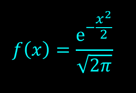
The case where μ = 0 and σ = 1 after computing the Z-scores is called the standard normal distribution.
Equation for the standard normal distribution is
The following is the plot of the standard normal probability density function.
Before using the Probability Density Function (PDF) toolkit, please ensure your dataset and workflow adhere to the following standards:
File Naming
Rename your CSV file according to the section you are analyzing:
CementAPCToolKit_RawMill.csv
CementAPCToolKit_CoalMill.csv
CementAPCToolKit_Kiln.csv
CementAPCToolKit_CementMill.csv
Header and Column Formatting
Single header row: Include descriptive labels for all dependent and independent variables.
No spaces: Use underscores instead of spaces (e.g., Elevator_Load
).
Rename feed column: Label the mill or kiln feed column as Total_Feed
.
Column order: Columns may appear in any order—no specific sequence is required.
Preprocessing
Follow the formatting exemplified in the provided screenshot (e.g., consistent decimal separators, no embedded units).
Browse and Upload
Click Select file and locate your preprocessed CSV.
Click Upload.
Run the Analysis
After upload completes, click Run to execute the Python analysis.
When prompted, specify the plant section—enter one of:
(Use the exact suffix matching your file name.)
Common issues:
Incorrect header formatting
Missing or misnamed Total_Feed
column
Spaces in column names
Need help?
Visit Contact → Fill the Contact Form, or
Email us directly at [email protected].
By following these guidelines, you’ll ensure seamless integration with the Cement APC Toolkit and obtain reliable PDF-based insights.